S3 Data Fetching Techniques
In object-storage-native database architectures (such as Turbopuffer), achieving sub-100 millisecond search latencies requires fetching data from Amazon S3 into local NVMe SSD caches — over the network, one block at a time. The question that shapes the entire I/O design is: how many bytes should each fetch grab?
The answer is unintuitive: as many as you reasonably can, because the cost of a fetch is almost entirely fixed overhead.
What Block Size Is
Block size () is the contiguous chunk of bytes (e.g., , , ) in which data is grouped, fetched, and cached — rather than reading individual bytes or downloading full multi-gigabyte index files.
[S3 Object Storage]
  ~$0.02/GB | ~500ms
        │
        │  Block Range Fetch (16 KB ... 1 MB)
        ▼
[Local NVMe SSD]
  ~$0.10/GB | ~100ms
The Latency Equation
The total latency () to retrieve a block over HTTP/S3 is governed by:
Where:
- is the fixed HTTP/TCP round-trip latency to S3 () — paid on every call, regardless of size.
- is the payload size in bytes.
- is the single-connection S3 network throughput ().
The critical observation: the two terms are wildly asymmetric. The round-trip is measured in milliseconds; the transfer term for reasonable block sizes is measured in microseconds.
Fetching 8× More Bytes, Paying ~1% More
Comparing a fetch against a fetch:
An larger payload costs only extra — a increase in total latency.
The pattern holds across the board:
| Payload Size | Transfer Time | Total Latency | vs. 16 KB |
|---|---|---|---|
| — | |||
The Key Insight
Because fixed network round-trip costs () dominate small reads, each additional byte fetched is nearly free — until the transfer term grows to the scale of the round-trip itself. Doubling your block size is almost always a better trade than doubling your number of requests: two calls for cost , while one call for costs .
The corollary: the only real cost of a larger block is cache pollution — fetching bytes you'll never read into the NVMe cache. The cost of a smaller block is another full round-trip. That asymmetry — round-trips are expensive, bytes are cheap — is the foundational lever behind object-storage-native I/O design.
Levers to Pull to Maximize Speed of Access from S3 (to NVMe)
Lever 1: Massive Parallel Range Requests
What is an S3 Range Request?
An HTTP Byte-Range Request allows a client to request only a specific slice of bytes from an object stored in Amazon S3 (or any HTTP/1.1-compliant object store) rather than downloading the entire file.
In traditional database architectures, accessing a table or index requires downloading or hydrating multi-gigabyte files to disk. In contrast, object-storage native engines (like Turbopuffer) store large SSTables or vector cluster files on S3, but only fetch exact byte offsets—such as a 32 KB index block at the end of a file or a 128 KB vector chunk—directly over the wire.
Real S3 API Call Examples
-
Raw HTTP Request Header:
httpGET /vector-data/cluster_79.bin HTTP/1.1 Host: my-bucket.s3.amazonaws.com Range: bytes=1048576-1179647 Authorization: AWS4-HMAC-SHA256 ...(The
Range: bytes=1048576-1179647header instructs S3 to return exactly 128 KB starting at offset 1 MB). -
cURL Command:
bashcurl -r 1048576-1179647 \ -H "Host: my-bucket.s3.amazonaws.com" \ https://my-bucket.s3.amazonaws.com/vector-data/cluster_79.bin \ -o chunk_42.bin -
AWS SDK (
@aws-sdk/client-s3) API Call:typescriptimport { S3Client, GetObjectCommand } from "@aws-sdk/client-s3"; const s3 = new S3Client({ region: "us-east-1" }); // Requesting a specific 128 KB byte range const response = await s3.send( new GetObjectCommand({ Bucket: "my-vector-bucket", Key: "cluster_79.bin", Range: "bytes=1048576-1179647", // Start-End inclusive }), ); const chunkBytes = await response.Body!.transformToByteArray();
What is Drive I/O Depth (Queue Depth)?
Drive I/O Depth (also called Queue Depth) refers to the number of concurrent, outstanding read/write operations queued or in-flight simultaneously between the application CPU, network stack, and storage controller.
Why High I/O Depth is Necessary for S3 and NVMe
- Single Connection Bottleneck: A single HTTP stream/connection to S3 caps out at roughly ~100 MB/s due to TCP windowing and latency bounds. However, modern cloud instances (e.g., AWS EC2) feature 50 Gbps to 100 Gbps network cards.
- Flat Latency Profile: S3 round-trip P90/P99 latency sits around 50–100 ms and varies very little whether you fetch 16 KB or 1 MB.
- Hardware Parallelism: Both cloud network hypervisors and local NVMe SSDs feature dozens of internal hardware queues/channels. Executing requests sequentially leaves over 90% of the hardware capacity idle.
- The Math of High Throughput: To saturate a 10 Gbps (1.25 GB/s) network link using 128 KB requests with 50 ms S3 latency:
Code Example: Maximizing Throughput with Parallel Range Requests
The following TypeScript code uses native fetch to execute 64 concurrent byte-range requests across a large file on S3, maintaining a high I/O queue depth to maximize bandwidth saturation:
const CHUNK_SIZE = 128 * 1024; // 128 KB blocks
const CONCURRENCY_LIMIT = 64; // High I/O Queue Depth

/** Issues a single async HTTP Byte-Range request. */
async function fetchByteRange(
  url: string,
  startByte: number,
  endByte: number,
): Promise<Uint8Array> {
  const response = await fetch(url, {
    headers: { Range: `bytes=${startByte}-${endByte}` },
  });
  return new Uint8Array(await response.arrayBuffer());
}

/** Saturates network throughput by executing concurrent range requests. */
async function parallelS3Download(
  objectUrl: string,
  totalBytes: number,
  chunkSize = CHUNK_SIZE,
  concurrencyLimit = CONCURRENCY_LIMIT,
): Promise<void> {
  // Generate list of byte offsets
  const byteRanges: Array<[number, number]> = [];
  for (let start = 0; start < totalBytes; start += chunkSize) {
    byteRanges.push([start, Math.min(start + chunkSize - 1, totalBytes - 1)]);
  }

  // Worker pool: keeps exactly `concurrencyLimit` requests in flight,
  // limiting memory while keeping I/O depth high
  let nextIndex = 0;
  const chunkSizes: number[] = new Array(byteRanges.length);

  async function worker(): Promise<void> {
    while (nextIndex < byteRanges.length) {
      const i = nextIndex++;
      const [start, end] = byteRanges[i];
      const data = await fetchByteRange(objectUrl, start, end);
      chunkSizes[i] = data.length;
    }
  }

  const startTime = performance.now();
  await Promise.all(
    Array.from({ length: concurrencyLimit }, () => worker()),
  );
  const elapsed = (performance.now() - startTime) / 1000;

  const downloadedBytes = chunkSizes.reduce((sum, size) => sum + size, 0);
  const throughputMbps = downloadedBytes / (1024 * 1024) / elapsed;

  console.log(
    `Fetched ${byteRanges.length} chunks ` +
      `(${(downloadedBytes / (1024 * 1024)).toFixed(2)} MB) ` +
      `in ${elapsed.toFixed(3)}s | Throughput: ${throughputMbps.toFixed(2)} MB/s`,
  );
}

// Example usage (Fetching a 64 MB file split into 512 x 128 KB range requests,
// with 64 in flight at any given time):
// parallelS3Download(
//   "https://my-bucket.s3.amazonaws.com/large_file.bin",
//   64 * 1024 * 1024,
// );
Lever 2: Direct Byte-Range Fetches (Metadata & Index Blocks)
What are Direct Byte-Range Fetches for Metadata?
In traditional databases (like MySQL or Elasticsearch), accessing a table or index often requires downloading, hydrating, or memory-mapping full multi-gigabyte SSTables or index files into local disk storage before executing queries.
In an object-storage-native architecture (for ex: Turbopuffer), SSTables and vector cluster files on S3 can be gigabytes large. Instead of downloading these massive files in their entirety, the engine structures its file layout so that index blocks, key offsets, and bloom filters (metadata footers) sit at the end of the file (typically the last 32 KB or 64 KB).
By issuing precise byte-range requests directly to these index footers, the engine can inspect the internal layout of a multi-gigabyte file over the wire, pinpoint the exact byte offsets where the requested vector or key lives, and fetch only those specific data blocks.
How the 3-Step Fetch Chain Works
An LSM-based storage engine coordinates this using a structured 3-phase lookup chain to minimize data transfer. (The footer-fetch concept is broadly applicable — columnar formats like Parquet place metadata in footers too — but the specific 3-round chain below is Turbopuffer's implementation):
[S3 Object Store]
  │
  ├─ 1. Namespace Manifest (lsm.json)
  │     └─▶ Identifies relevant SSTable file UUIDs
  │
  ├─ 2. File Footer (Last 32 KB)
  │     └─▶ Parses key ranges & exact data block offsets
  │
  └─ 3. Data Block (128 KB Payload)
        └─▶ Retrieves target vectors / document records
- Round 1 — Manifest Lookup: The query engine inspects the namespace metadata (e.g.,
lsm.jsonor cached manifests) to determine which large SSTable files contain the requested key ranges or cluster IDs. - Round 2 — Index Block Range Request: The engine issues an S3 range request for the last 32 KB or 64 KB of the target SSTable file. This lightweight footer contains the sparse index mapping keys or vector IDs to physical byte offsets inside the file.
- Round 3 — Targeted Data Payload Request: Using the exact byte offsets extracted from the index footer, the engine issues a third range request to pull only the specific 128 KB data block containing the desired records.
Real S3 API Example: Suffix Byte-Range Requests
S3 supports negative/suffix byte ranges (e.g., bytes=-32768), which instruct the server to return the last bytes of an object regardless of the file's total size:
-
S3 HTTP Request Header (Reading the 32 KB Footer):
httpGET /namespaces/cursor_codebase/sstable_9f82a.bin HTTP/1.1 Host: my-bucket.s3.amazonaws.com Range: bytes=-32768 -
cURL Command:
bashcurl -r -32768 \ https://my-bucket.s3.amazonaws.com/sstable_9f82a.bin \ -o footer_32k.bin
Code Example: Footer Inspection & Targeted Fetch
The following TypeScript code demonstrates how to fetch a file footer, parse a target byte offset, and issue a second targeted byte-range request to retrieve only the required data block:
import { S3Client, GetObjectCommand } from "@aws-sdk/client-s3";

const s3 = new S3Client({ region: "us-east-1" });
const BUCKET = "my-vector-bucket";
const KEY = "namespaces/tenant_101/sstable_42.bin";

// STEP 1: Fetch the last 32 KB (32,768 bytes) of a 2 GB file
const footerResponse = await s3.send(
  new GetObjectCommand({
    Bucket: BUCKET,
    Key: KEY,
    Range: "bytes=-32768", // Suffix range: last 32 KB
  }),
);
const footerBytes = await footerResponse.Body!.transformToByteArray();

// STEP 2: Parse the footer (Example: extracting offset & length of Block #7)
// Assuming a binary format where the last 8 bytes store [block_offset, block_length]
const view = new DataView(
  footerBytes.buffer,
  footerBytes.byteOffset,
  footerBytes.byteLength,
);
const blockOffset = view.getUint32(footerBytes.length - 8, false); // big-endian
const blockLength = view.getUint32(footerBytes.length - 4, false); // big-endian

console.log(
  `Target data block located at offset ${blockOffset} with length ${blockLength} bytes.`,
);

// STEP 3: Issue a targeted range request for ONLY that 128 KB block
const dataResponse = await s3.send(
  new GetObjectCommand({
    Bucket: BUCKET,
    Key: KEY,
    Range: `bytes=${blockOffset}-${blockOffset + blockLength - 1}`,
  }),
);
const targetBlockBytes = await dataResponse.Body!.transformToByteArray();

console.log(
  `Successfully retrieved ${targetBlockBytes.length} bytes of vector data ` +
    `without downloading the full SSTable.`,
);
Architectural Trade-offs
- The Benefit: Saves downloading gigabytes of unneeded vector or full-text data over the network, keeping S3 bandwidth costs and memory usage extremely low.
- The Penalty: Incurs an additional S3 round-trip latency overhead (~50–100 ms) to fetch the index block before fetching the data.
- The Mitigation: Object-storage-native engines (for ex: Turbopuffer) cache small metadata footers (
lsm.jsonand index footers) aggressively in DRAM and NVMe SSDs. Once the metadata footer is cached locally, queries bypass Round 1 and Round 2 completely, executing in a single I/O fetch directly to disk or S3.
Lever 3: Zero-Copy Deserialization (rkyv / archive)
What is Zero-Copy Deserialization?
In high-throughput database systems, fetching data over the network or reading it from an NVMe SSD is only half the battle. Once bytes land in memory, traditional databases pay a steep "deserialization tax":
- Traditional Deserialization (JSON, Protobuf, BSON): The CPU must parse the incoming byte stream, validate schemas, allocate new heap memory, and copy fields one-by-one into native programming language objects (e.g., converting ASCII strings or packed byte arrays into native structs). When reading gigabytes of vector data per second, this CPU decoding loop and memory allocation churn quickly become the primary bottleneck.
- Zero-Copy Deserialization (
rkyv/archive): The data is written to S3 or disk in the exact binary memory layout that the CPU expects in native Rust structs. Once the bytes land in user-space DRAM, the application casts the byte buffer pointer directly to a native reference (e.g.,&ArchivedVectorBlock). No heap memory is allocated, and no bytes are copied or re-interpreted.
How Object-Storage-Native Engines Use rkyv for Vector Search
Object-storage-native engines (for ex: Turbopuffer) use the open-source Rust library rkyv (also referred to as archive) to structure SSTable files and RaBitQ vector blocks on S3:
- Direct Buffer Projection: When 128 KB byte-range requests land in memory from S3 or the NVMe SSD, the query engine casts the memory buffer directly to Rust structs with zero CPU translation cycles.
- Immediate Register Math: Because the stored byte layout matches the target CPU register alignment, the CPU immediately begins evaluating hardware-accelerated SIMD bitwise
ANDandpopcountoperations directly on the memory-mapped bytes. - Bandwidth-Bound Throughput: By removing the deserialization tax, CPU utilization stays near zero during file loading, shifting the performance ceiling entirely to network and NVMe hardware limits.
Conceptual Code Comparison: Traditional vs. Zero-Copy
Traditional Approach (Protobuf / JSON Parsing — Slow)
// Traditional: Allocates new heap memory for every vector field
struct VectorBlock {
    ids: Vec<u64>,
    bitmasks: Vec<u8>,
    correctors: Vec<f32>,
}

fn process_traditional(network_bytes: &[u8]) {
    // CPU-bound: parses byte stream, allocates heap arrays,
    // and copies memory
    let block: VectorBlock = serde_json::from_slice(network_bytes).unwrap();

    // Perform search on newly allocated heap memory
    evaluate_math(&block);
}
Zero-Copy Approach (rkyv / archive — Instant)
use rkyv::{archived_root, Archive, Serialize};

#[derive(Archive, Serialize)]
struct VectorBlock {
    ids: [u64; 256],
    bitmasks: [u8; 4096], // 128-bit RaBitQ codes for 256 vectors
    correctors: [f32; 256],
}

fn process_zerocopy(network_bytes: &[u8]) {
    // Zero-Copy: projects pointer addresses directly onto
    // network bytes. 0 allocations, 0 memory copies, 0 parsing loops.
    let block = unsafe { rkyv::archived_root::<VectorBlock>(network_bytes) };

    // Direct pointer access into network buffer!
    let first_id = block.ids;
    let first_corrector = block.correctors;
}
Architectural Trade-offs
| Advantage | Trade-off / Penalty |
|---|---|
| Instant Data Readiness: Data is queryable the exact microsecond it lands in DRAM. | Strict Byte Alignment: Endianness and memory alignment must match the target CPU architecture. |
| Zero Memory Churn: Eliminates garbage collection stalls and heap allocator lock contention. | Custom Format Maintenance: Requires owning the binary serialization format rather than relying on standard tools like Apache Parquet. |
| Maximized CPU Efficiency: Frees up CPU cycles exclusively for vector distance calculation. | Validation Overhead: Must run lightweight validation checks to ensure untrusted network buffers don't cause out-of-bounds pointer reads. |
Lever 4: Speculative Pre-fetching & Cache Warming (hint_cachewarm)
What is Speculative Pre-fetching & Cache Warming?
In an object-storage native database, a cold query that misses both DRAM and NVMe SSD caches must pull data directly from S3, incurring a latency of 500 ms to 1 second. To eliminate this cold-start penalty during user interactions, object-storage-native engines (for ex: Turbopuffer) use two complementary mechanisms:
- Speculative Pre-fetching (Engine Level): Rather than waiting for a sequential chain of read dependencies, the database engine continuously predicts down-chain data needs based on query plans and speculatively fires off parallel byte-range requests to S3 before the CPU explicitly requests them.
- Cache Warming (
hint_cachewarm— API Level): An explicit application primitive exposed to client applications (analogous to the POSIXmadvise/posix_fadvisesystem call). When an end-user opens a UI panel (such as clicking on a search bar or opening an AI Q&A pane in Notion), the client app fires ahint_cachewarmrequest. By the time the user finishes typing their search query milliseconds later, the relevant namespace index blocks are already hydrated from S3 into NVMe SSD / DRAM caches, dropping query latency down to 10–20 ms. (Engine-level speculative prefetching is a broadly applicable technique — but the explicit client-facinghint_cachewarmAPI primitive itself is Turbopuffer-specific.)
How hint_cachewarm Works Under the Hood
[Client UI Event]           [Query Engine]           [Storage Tiers]
(user opens search pane)
   │
   ├─ 1. POST /v1/namespaces/{tenant}/warm_cache
   │     (Fires before user types a single character)
   │
   └────▶ Checks DRAM / NVMe cache
             │
             ├─ Cache Hit ──▶ Free call (0 compute cost)
             │
             └─ Cache Miss ──▶ Triggers parallel S3 range
                               fetches; hydrates the
                               NVMe ring buffer
- Cost Model: If the target namespace metadata and vector blocks are already hot in cache, the
hint_cachewarmcall is completely free. If cold, the provider (for ex: Turbopuffer) charges for a single query to cover the cost of hydrating the data from S3. - Speculation in Action: During search execution, while the CPU is evaluating candidate clusters, the query engine speculatively issues read requests for adjacent leaf-node blocks or full-text posting lists before the primary evaluation loop finishes.
Code Example: Triggering hint_cachewarm in Client Workflows
HTTP API Call (cURL)
curl -X POST \
     "https://api.example-db.com/v1/namespaces/workspace_42/warm_cache" \
     -H "Authorization: Bearer tpk_live_..." \
     -H "Content-Type: application/json"
TypeScript Client Example
const API_KEY = "tpk_live_sample_key";
const BASE_URL = "https://api.example-db.com/v1";

/**
 * Fires an asynchronous cache warming hint when a user
 * focuses on a search bar. Pre-hydrates cold S3 data into
 * NVMe/DRAM before the user submits a query.
 */
async function hintCacheWarm(namespaceId: string): Promise<void> {
  const url = `${BASE_URL}/namespaces/${namespaceId}/warm_cache`;

  try {
    const response = await fetch(url, {
      method: "POST",
      headers: {
        Authorization: `Bearer ${API_KEY}`,
        "Content-Type": "application/json",
      },
    });

    if (response.ok) {
      console.log(
        `[CacheWarm] Successfully triggered warming for ${namespaceId}`,
      );
    } else {
      console.warn(`[CacheWarm] Warning: Returned status ${response.status}`);
    }
  } catch (error) {
    // Cache warming is non-blocking; failures should never break the UI
    console.warn(`[CacheWarm] Failed to send hint: ${error}`);
  }
}

/** Simulates a UI event handler when a user clicks into a search box. */
async function onUserSearchFocus(tenantWorkspace: string): Promise<void> {
  // Pre-warm the cache immediately on focus
  await hintCacheWarm(tenantWorkspace);
}

// Example usage:
// onUserSearchFocus("workspace_cursor_codebase");
Architectural Trade-offs
| Advantage | Trade-off / Penalty |
|---|---|
| Sub-20ms User Experience: Eliminates S3 tail-latency spikes (~1s) for interactive user queries. | Bandwidth Waste on Aborted Searches: If a user opens a search modal but closes it without typing, bandwidth was spent fetching cold S3 blocks. |
| Free for Hot Data: Costs nothing if the namespace is already cached in DRAM or local NVMe. | Cache Eviction Pressure: Pre-warming an inactive tenant can evict active blocks belonging to other tenants from the FIFO ring buffer. |
Lever 5: Sequential FIFO Ring Buffer on NVMe
What is a Sequential FIFO Ring Buffer on NVMe?
When fetching blocks from S3 to cache locally on an NVMe SSD, traditional databases often create thousands of individual files across a standard file system directory (e.g., /cache/tenant_1/block_42.bin).
Object-storage-native engines (for ex: Turbopuffer) bypass file system complexity by pre-allocating one single file that spans the entire capacity of the physical NVMe SSD. The engine then operates on this giant file as a continuous, circular First-In, First-Out (FIFO) ring buffer.
As new 128 KB data blocks arrive from S3, the engine writes them sequentially into the buffer at the current write offset. When the write pointer reaches the physical end of the drive, it simply wraps back around to offset 0 and overwrites the oldest cached data at the tail. (This is a broadly applicable technique — Kafka's log segments and database commit logs use the same pre-allocated sequential-write pattern.)
[Pre-Allocated NVMe File: e.g., 1 TB Disk Capacity]
┌──────────────────────────────────────────────────────┐
│ Block 101 │ Block 102 │ ... │ Block 90 │ Block 91 │… │
└──────────────────────────────────────────────────────┘
             ▲                        ▲
             │                        │
      Tail (Oldest Data)   Write Pointer (New S3 Fetch)
Why This Eliminates Filesystem Stalls & Maximizes Speed
- Zero Metadata & Journaling Overhead: Traditional OS file systems (like
ext4orxfs) suffer from directory lock contention, inode allocation delays, and journalfsyncstalls when rapidly creating and deleting millions of small files. Operating on a single pre-allocated file eliminates these kernel-level locks. - Saturating Sequential NVMe Write Speeds: Modern NVMe SSD flash controllers are physically optimized for continuous sequential writes. Random small-file creation forces the SSD's internal controller into expensive background Garbage Collection (GC) erase cycles, causing latency spikes. Sequential ring buffer writes allow the drive to sustain peak hardware write throughput.
- Minimal, Rock-Solid Codebase: Because the cache logic does not need complex tree-based eviction indices or garbage collection heuristics, this entire NVMe caching layer can be implemented in a very small footprint — for ex: Turbopuffer's founder implemented it in ~200 lines of rock-solid Rust.
Rust Conceptual Code: Pre-Allocated FIFO Ring Buffer
The following Rust snippet demonstrates how a fixed-size file on NVMe can be written sequentially as a circular FIFO ring buffer:
use std::fs::{File, OpenOptions};
use std::io::{self, Seek, SeekFrom, Write};
use std::sync::atomic::{AtomicU64, Ordering};

pub struct NvmeFifoRingCache {
    file: File,
    capacity_bytes: u64,
    write_head: AtomicU64, // Monotonically increasing byte position
}

impl NvmeFifoRingCache {
    /// Opens or pre-allocates a single file spanning the disk.
    pub fn new(disk_path: &str, capacity_bytes: u64) -> io::Result<Self> {
        let file = OpenOptions::new()
            .read(true)
            .write(true)
            .create(true)
            .open(disk_path)?;

        // Pre-allocate full file size on NVMe to prevent
        // filesystem fragmentation
        file.set_len(capacity_bytes)?;

        Ok(Self {
            file,
            capacity_bytes,
            write_head: AtomicU64::new(0),
        })
    }

    /// Writes a 128 KB block sequentially, wrapping at capacity.
    pub fn write_block(&mut self, data: &[u8]) -> io::Result<u64> {
        let block_len = data.len() as u64;

        // Fetch current global position and increment atomically
        let current_pos = self
            .write_head
            .fetch_add(block_len, Ordering::SeqCst);

        // Calculate physical circular offset on disk
        let physical_offset = current_pos % self.capacity_bytes;

        // Seek and write directly into the pre-allocated buffer
        self.file.seek(SeekFrom::Start(physical_offset))?;
        self.file.write_all(data)?;

        Ok(physical_offset)
    }
}
Architectural Trade-offs
| Advantage | Trade-off / Penalty |
|---|---|
| Maximized NVMe Write Speed: Sustains continuous multi-gigabyte/sec write throughput without triggering SSD garbage-collection stalls. | Risk of Overwriting Hot Blocks: Naive FIFO ring buffers overwrite the oldest blocks regardless of popularity. (Engines can add heuristics to skip/protect heavily accessed active blocks from being eaten). |
| Zero Memory/OS Overhead: Eliminates inode locks, file system fragmentation, and metadata journal syncs. | Ephemeral Storage Only: Data in the NVMe ring buffer is non-durable and completely lost if the VM restarts. (Acceptable because S3 remains the authoritative source of truth). |
| Ultra-Low Complexity: Entire storage engine cache requires ~200 lines of Rust code. | Fixed Disk Allocation: Disk capacity must be pre-allocated upfront on instance boot. |
Industry Takes
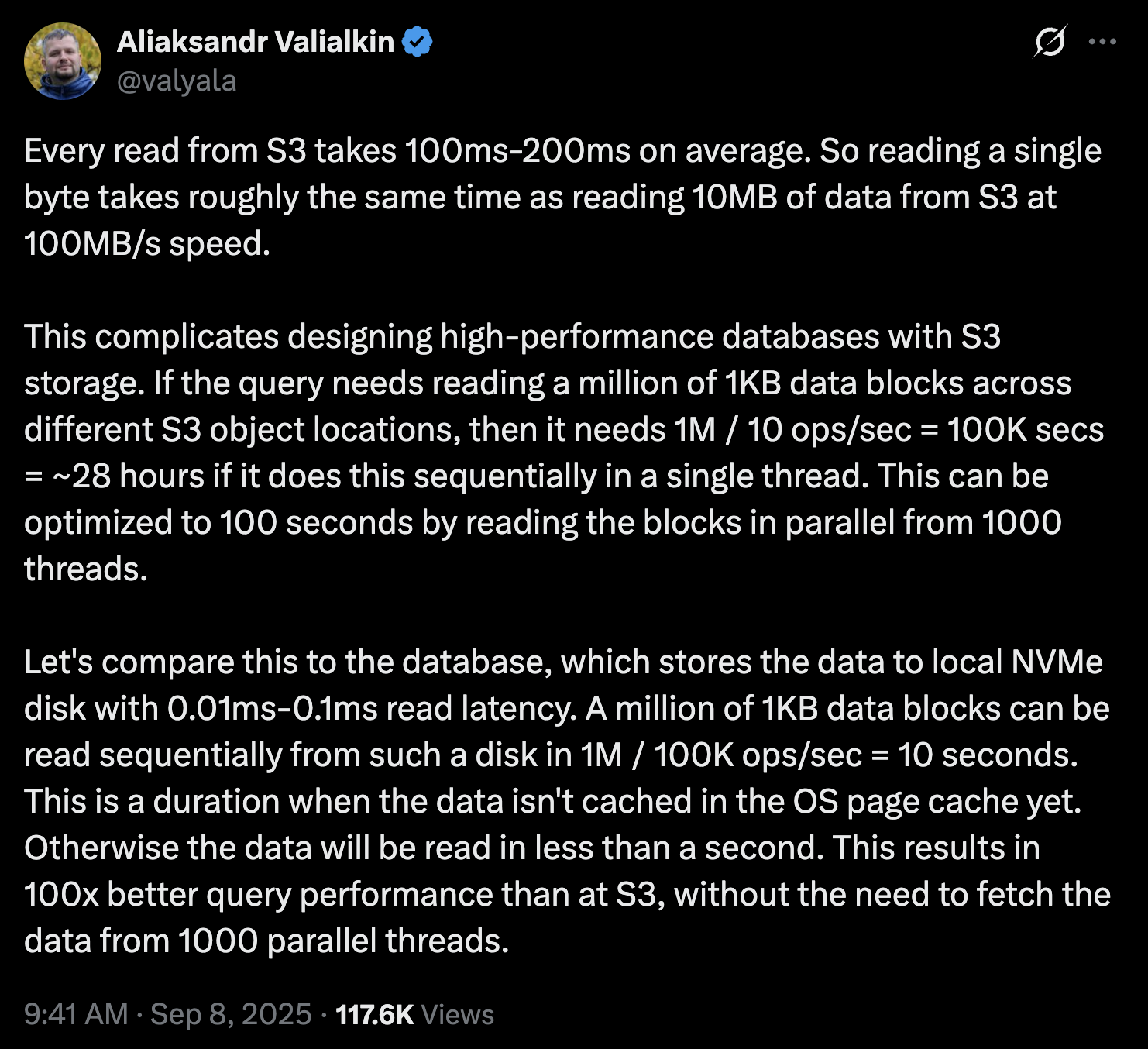
Source: Aliaksandr Valialkin on X
Related reads
- NVMe SSDs — the ephemeral local flash tier this blog caches into
- DRAM — the most expensive tier at the top of the pipeline
- Accessing DRAM & NVMe SSDs in the Cloud — how (and how not) code reaches these tiers
- SSTables: The Sorted String Table — the immutable files being fetched over byte ranges